Basic GWAS Plots

gwasplot provides fast Manhattan and QQ plots for GWAS summary statistics. This vignette walks through the core plotting workflow using simulated data — no real GWAS files or DuckDB connections required.

Simulate data

The helper below generates a data frame with standard columns CHROM, POS, and PVALUE, distributing variants proportionally across chromosomes and optionally injecting genome-wide significant signals.

library(gwasplot)
#> ℹ Setting duckdb_max_memory to 7GB, using 80% of available system memory.
#> ℹ Change this with options(duckdb_max_memory = 'XGB')
#> 
#> Attaching package: 'gwasplot'
#> The following object is masked from 'package:stats':
#> 
#>     qqplot

# Approximate chromosome sizes (Mb, hg38)
chr_mb <- c(249, 242, 198, 190, 181, 171, 159, 145, 138, 134,
            135, 133, 115, 107, 102,  90,  83,  80,  59,  63, 47, 51)

sim_gwas <- function(n_total, hits = NULL,
                     chroms = paste0("chr", 1:22)) {
  sizes <- chr_mb[seq_along(chroms)]
  dfs <- Map(function(ch, mb) {
    n <- max(1L, round(n_total * mb / sum(sizes)))
    data.frame(
      CHROM  = ch,
      POS    = sort(sample.int(mb * 1e6L, n)),
      PVALUE = runif(n)
    )
  }, chroms, sizes)
  df <- do.call(rbind, dfs)
  for (h in hits) {
    idx <- df$CHROM == h$chrom & abs(df$POS - h$pos) < h$window
    df$PVALUE[idx] <- runif(sum(idx), h$pmin, h$pmax)
  }
  df
}

set.seed(42)
gwas_df <- sim_gwas(
  n_total = 500000,
  hits = list(
    list(chrom = "chr2",  pos = 135e6, window = 5e5, pmin = 1e-15, pmax = 1e-8),
    list(chrom = "chr5",  pos =  50e6, window = 5e5, pmin = 1e-12, pmax = 1e-8),
    list(chrom = "chr11", pos =  70e6, window = 5e5, pmin = 1e-20, pmax = 1e-8),
    list(chrom = "chr17", pos =  30e6, window = 5e5, pmin = 1e-10, pmax = 1e-8)
  )
)

head(gwas_df)
#>        CHROM   POS    PVALUE
#> chr1.1  chr1   611 0.4831109
#> chr1.2  chr1  1527 0.6988779
#> chr1.3  chr1  9474 0.8769163
#> chr1.4  chr1 28440 0.3938541
#> chr1.5  chr1 54879 0.7036494
#> chr1.6  chr1 58418 0.5482878

Genomic inflation factor

lambda_gc() computes the genomic inflation factor from the PVALUE column. A value close to 1 indicates well-controlled test statistics.

lambda_gc(gwas_df)
#> lambda_GC = 1.0007
#> [1] 1.000725

QQ plot

qqplot() accepts a numeric vector of p-values and returns a ggplot object, which renders inline in the document.

qqplot(gwas_df$PVALUE)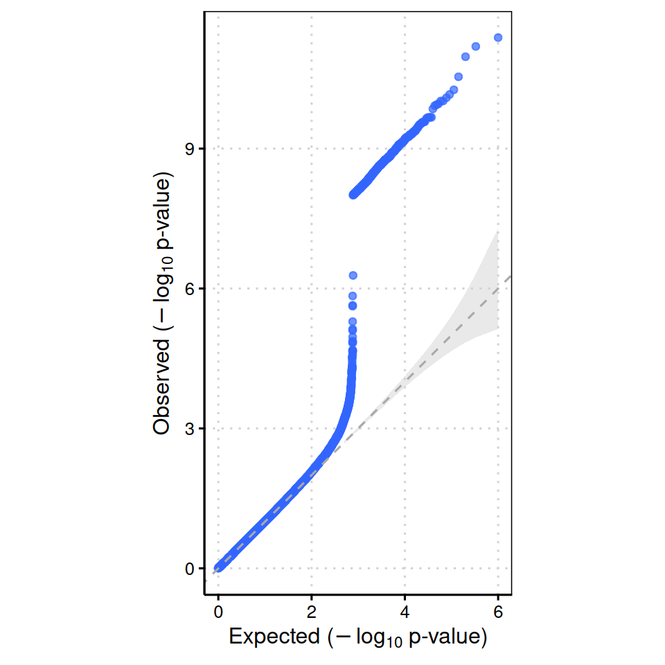

Manhattan plot

manhattan() saves the plot to a file via ggsave. Pass width, height, and dpi through ... to control output dimensions.

outfile <- knitr::fig_path(".png")
dir.create(dirname(outfile), showWarnings = FALSE, recursive = TRUE)
manhattan(gwas_df, output = outfile, width = 10, height = 4, dpi = 150, base_size = 14)
#> INFO [2026-02-25 22:54:26] Now preparing to plot
#> INFO [2026-02-25 22:54:26] Done preparing to plot 1168 SNPs.
#> Warning: The `size` argument of `element_line()` is deprecated as of ggplot2 3.4.0.
#> ℹ Please use the `linewidth` argument instead.
#> ℹ The deprecated feature was likely used in the gwasplot package.
#>   Please report the issue at <https://github.com/weinstocklab/gwasplot/issues>.
#> INFO [2026-02-25 22:54:26] Now rendering
#> INFO [2026-02-25 22:54:28] done plotting.
knitr::include_graphics(outfile)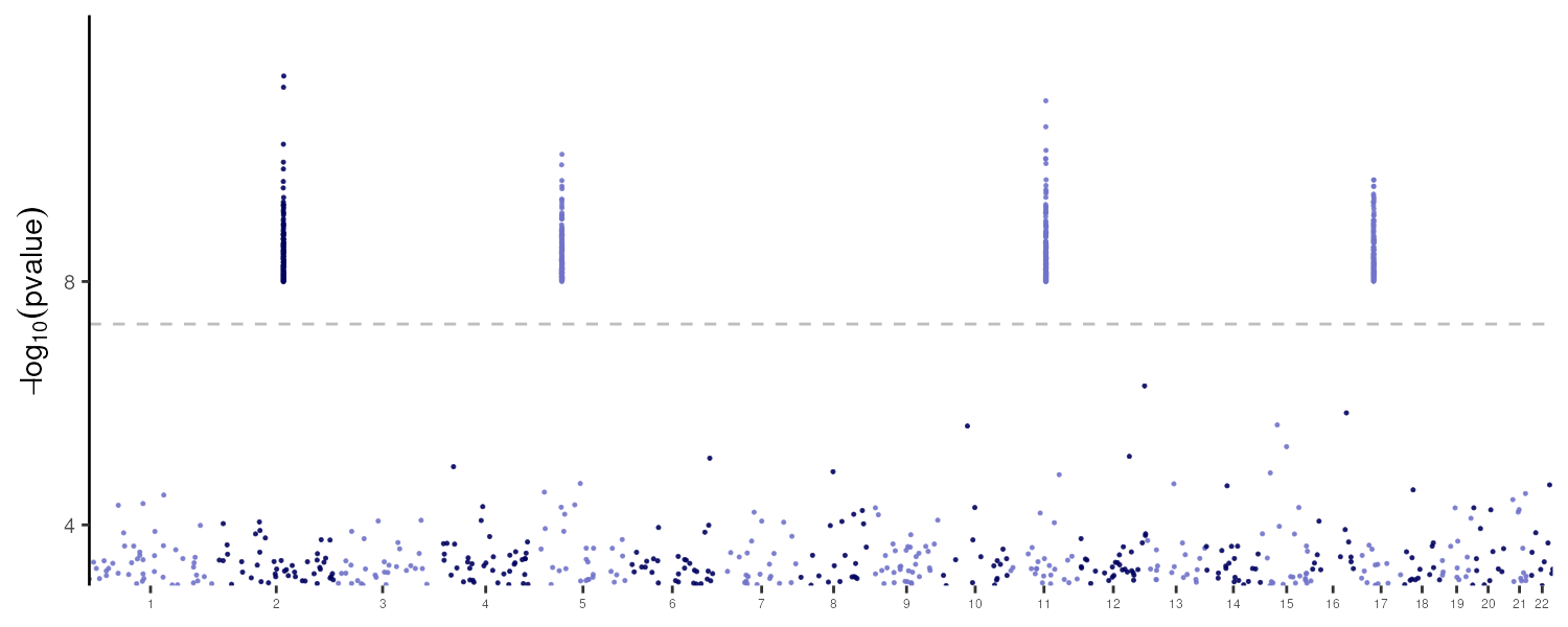

The four injected signals on chromosomes 2, 5, 11, and 17 are clearly visible above the genome-wide significance threshold (−log₁₀ p ≈ 7.3).